Exercise 1:
Goal
The goal of the exercise is to measure the distances that the ultrasonic sensor records with different distances and object/materiales.
Plan
We are going to use hard and soft materiales at different distances and measure the actual distance with a folding ruler.

Results
| Surface | Sensor value | Actual value |
| Soft | 42 | 42 |
| Soft | 79 | 78 |
| Medium | 80 | 78 |
| Medium | 42 | 41 |
| Hard | 43 | 42 |
| Hard | 78 | 78 |
Conclusion
The results contradict our expectations that the softer materiales would resolve in a larger difference between the measured and actual values. We expected that the softer materials would absorb the soundwaves and thus cause readings that would not be as accurate.
Exercise 2
Goal
To see if different sample intervals will affect the distance measured by the ultrasonic sensor.
Plan
The way we are doing to test this by keeping the distance to the object constant and conduct measurements with different sample intervals.
Result
While measuring we kept a constant distance of 17 cm.
| Sample interval | Measured Distance |
| 0 | 20 |
| 100 | 20 |
| 200 | 20 |
| 300 | 20 |
| 400 | 20 |
| 500 | 20 |
| 2000 | 20 |
Conclusion
As can be seen from the results it made no difference using different sample intervals. This means that the old minimum interval is no longer necessary, it might’ve been present in the older versions of lejOS due to the possibility of the sensor receiving an ultrasonic ping which it sent previously and thus getting a wrong reading.
Exercise 3
Goal
Our goal in this exercise is to examine if it’s possible to measure 254 cm and to see whether a lower sample interval will affect the measurement.
Plan
Our plan is to place the sensor towards a wall and move it away from the wall until we get a measurement of 254 cm, once we have that distance we will change the sample interval to be less than the time it takes to receive a echo. The time it takes sound to move 254 cm to wall and back again is 14.928 msec, which is calculated this way:
(2*distance to travel)/speed of sound ->
(2 * 2.54m)/340.29m/sec = 0.014928sec = 14.928msec.
Therefore we will set the sample interval to 5msec.
Result
Our observation was that there was no difference when using the short sample interval. This let to a discussion with Ole Caprani in which he pointed out to us that the code might hold the answer – that no ping can be made until the echo has been received.
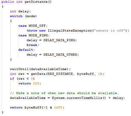
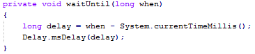
After having a look at the code below from the LeJOS UltrasonicSensor-class we can see that the system waits for atleast 30msec before making another ping, which is more than the minimum wait time calculated above. This means that the sample interval does not actually have an impact on measurements.
Conclusion
The sample interval doesn’t affect the practical usage of the sensor, it simply delays measurements (the default of the sample interval is 300msec, which makes the time between pings atleast 330msec, so about three times a second.)
Exercise 4
Goal
For this exercise the goal is to change the values of the constants in the code and observe what the changes does to the behaviour of the robot, and finally determine what kind of controller this is.
Plan
The way we go about this is by adjusting the value of one variable and leaving the other variables unchanged. By only working with one variable at a time we hope it will be easier to see what the variable controls and ultimately compare the results of changing the different constants to see which kind of controller it is.
Result
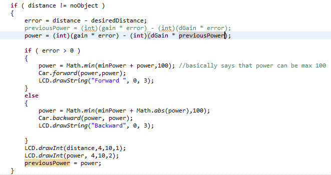
By changing the desiredDistance-variable in the program the only change in the behaviour we observed was that the distance to the object it found changed, the robot didn’t oscillate more or less around the point of the desiredDistance. On the other hand, changing the minPower-variable made the robot oscillate with larger amplitude around the specified desiredDistance.
Conclusion
From what we have observed we conclude that the controller in question is a PID controller, because the oscillation is larger when we increase the motor power.
Exercise 5
Goal
In the previous exercise we made the robot oscillate by just calculating the error between the current and desired point. Now we have to introduce the derivative term as described in [1].
Plan
Our plan is to follow the instruction in [1] and introduce the necessary new code in the class.
Result
With the derivative term introduced in the code, the robot still oscillates a little, but less compared to the original implementation.
Conclusion
By introducing the derivative term in the program for the robot we have achieved less oscillation in the robot around the point of the desired distance.
Exercise 6
Goal
To make a wall follower, using Philippe Hurbain’s concept for the RCX[2].
Plan
First off we have to remount the ultrasonic sensor to place it at a 45 degree angle to the forward facing direction of the robot, which will cause the measurements of distance for the robot to be small if it’s turning towards the wall, while becoming increasingly larger when turning away from the wall. Next we will have to program the robot to utilize the ultrasonic sensor to follow the wall – we are going to do that based on Philippe Hurbain’s program, although we’ll have to chance the constants proposed in his code since they are based on the raw 0-1023 interval while we only have a 0-255 interval (the raw value parsed to centimeters). We will try to get the appropriate values for the constants by doing empirical research of turning the robot towards and away from the wall, while measuring.
Result
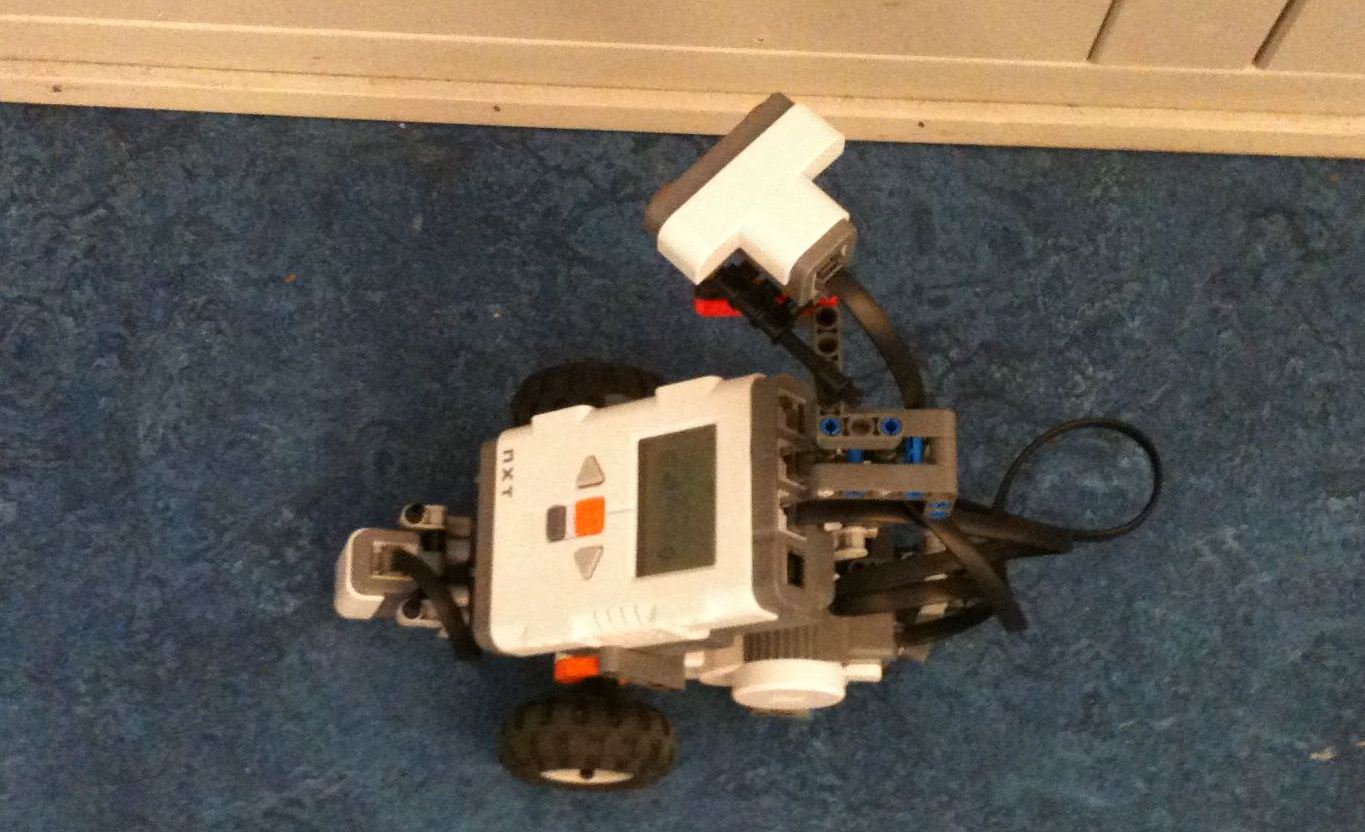


We found it problematic to get the appropriate values for the constants and had to change the positioning of the sensor because it would get very large increases in distances measured when turning away from the wall. We suspect this was because, by chance, the receiving part of the sensor was the part that was the furthest away from the wall and thus a slight turn meant a larger increase in the angle to the wall.
Conclusion
We didn’t get the robot to work very well, but the concept did work. Compare to Fred G. Martin’s algorithm[1] the major differences are that we have five different states and Martin’s only three, the smoothing of Martin’s algorithm – 50% on one wheel and 100% on the other – can be compared to the two extra states in our program in which we let the wheel float. We still stop one of the wheels if we either get too close or too far from the wall to increase the turning angle.
References
[1] Martin, Fred G. Robotic Explorations – A Hands-On Introduction to Engineering
[2] Philippe Hurbain, http://www.philohome.com/wallfollower/wallfollower.htm